The spin glass problem was first manifested in experiments on random magnets, and the Edwards-Anderson model was subsequently proposed. Since then, the simplicity of the model and the fundamental nature of the problem have been encouraging a great deal of effort to be invested on its study. While we confirmed the existence of the spin-glass phase transition in three dimensions by means of Monte Carlo simulations [1], the nature of the spin glass phase is a subject of active debates even today. Early theoretical works produced two paradigms that are consistent with experimental findings: the mean-field picture and the droplet picture. Investigations in the last two decades have been focused on the question as to which paradigm is correct for the three-dimensional model. For solving this problem, the principal tool was numerical calculations. It did not take too long, however, for researchers to realize the difficulty of the problem from the computational point of view. Even a mathematically rigorous statement was made: the problem of finding the ground-state of a given sample of the Edwards-Anderson spin glass model is NP-hard if the lattice is three dimensional or higher. Today’s largest system size that can be handled with conventional methods does not exceed L=30 for three-dimensional models, which is not enough to answer the question beyond reasonable doubts.

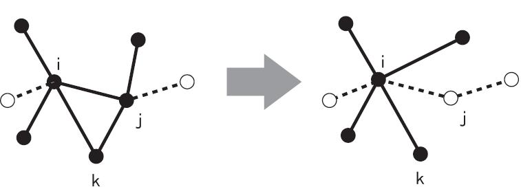
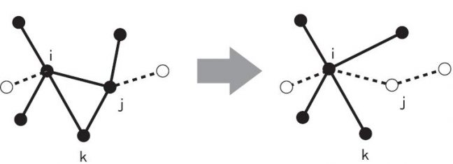
We proposed an approximate solution to the problem [2] based on recursive deformation. One of the most well-known examples for methods of this kind is the Migdal-Kadanoff (MK) real space renormalization, which yields a raasonably accurate result for the ferromagnetic Ising model and was applied later to spin glasses. Our approximation procedure consists of repeated application of an elementary operation (“contraction”) to the model with a given lattice geometry and the system size. As depicted in Fig.1, a contraction is performed as reconnection of bonds and recalculation of the bond strength. Starting from the the finite lattice on which the model is defined, we gradually deform it by contraction until it becomes a tree with no loop. Once the lattice has been deformed into a tree, it is easy to compute the correlation functions because of the absence of loops. In this way, we can treat much larger systems than we can with conventional numerical methods such as the Monte Carlo simulation.

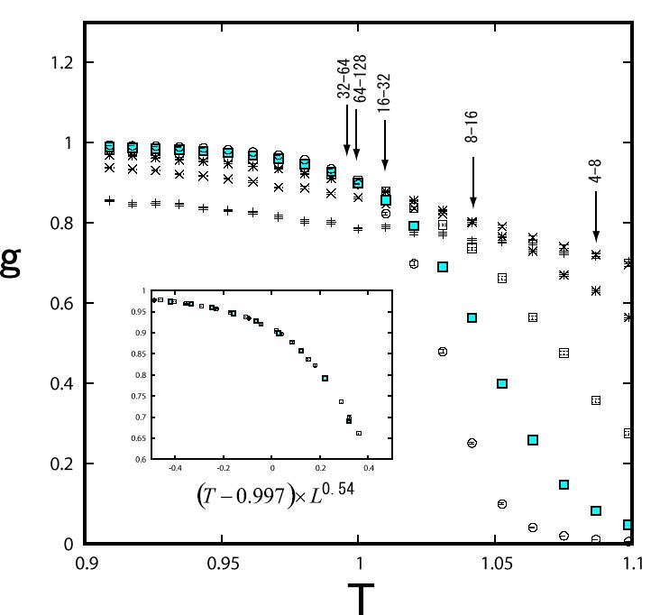
For the three dimensional system, the spin glass susceptibility shows a drastic change near T=J, which is presumably the transition temperature. This is confirmed by Fig.2, which shows the temperature dependence of the Binder parameter and the finite-size-scaling plot based on it. Curves of various system sizes cross each other and the crossing between larger systems takes place at lower temperature. The crossing point in the thermodynamic limit is located around T = 1.0 J and g = 0.9. We can also produce a finite-size-scaling plot that looks reasonable, as shown in the inset. The plot yields the estimates of the critical exponent; \(\nu=1.85\). The agreement of these values with the results of Monte Carlo simulation [3], Tc = 0.98(5) and \(\nu= 2.00 (15)\), are remarkably good considering the crudeness of the present approximation. This is also an improvement on the MK result [4], Tc = 0.39 and \(\nu=2.8\).
(by Naoki Kawashima)
References
[1] N. Kawashima and A. P. Young: “Phase transition in the three-dimensional \(\pm J\) Ising spin glass”, Phys. Rev. B 53 (1996) R484.[2] N. Kawashima: “Tree approximation for spin glass models”, J. Phys. Soc. Jpn. 25 (2006) 073002.
[3] E. Marinari, G. Parisi and J. J. Ruiz-Lorenzo: “Phase structure of the three-dimensional Edwards-Anderson spin glass”, Phys. Rev. B 58 (1998) 14852.
[4] B. W. Southern and A. P. Young: “Real space rescaling study of spin glass behavior in 3 dimensions”, J. Phys. C 10 (1977) 2179.
